The Uncertainty Principle Has a Sharpe Ratio: Quantum Portfolio Optimization in C++

Proposition

Quantum portfolio optimization does not require a quantum-native system. It requires a production-grade classical system with a quantum boundary condition. C++ is the only language positioned to satisfy both simultaneously.

This claim appears false at first inspection. The quantum computing ecosystem is Python: Qiskit, Ocean SDK, Cirq, Jupyter Notebooks, etc. Every tutorial begins with pip install qiskit. Every demo ends before deployment. This is not accidental. Python optimizes for research velocity. Production trading systems optimize for determinism, bounded latency, and operational survivability under pathological conditions. Research velocity is not on that list.

The industry mistake is therefore predictable: "If quantum finance exists in Python, then production quantum finance must also be Python." This inference is invalid. The actual problem is not: can Python call a quantum solver? That problem was solved years ago.

The actual problem is: Can quantum optimization be integrated into production financial infrastructure without rewriting the infrastructure itself?

That problem remains mostly unsolved. This post is an attempt.

Given Constraints

Let S = production financial systems
Let Q = practical quantum optimization tooling Let B(S,Q) = the boundary layer connecting them

Empirically: S ≈ C/C++ Q ≈ Python

Therefore: S ∩ Q → ∅

Not because quantum optimization is impossible. Because nobody built B(S,Q) correctly.

Null hypothesis H₀: A quantum optimizer cannot be integrated into a production C++ portfolio system without architectural compromise or systemic rewrite.

This project treats H₀ as an engineering target. Not a philosophical objection. Not a market thesis.

A falsifiable systems claim. This project refutes H₀. The evidence follows.

Methodology

The Language Decision

The obvious implementation path is wrong.

One could:

1. Write the optimizer in Python
2. Wrap Qiskit directly
3. Use NumPy for covariance computation
4. Produce benchmark graphs
5. Declare victory

This proves only that Python libraries can call other Python libraries. It does not solve the integration problem. Production trading infrastructure does not disappear merely because a notebook executed successfully. The system that matters — risk engines, execution infrastructure, portfolio accounting, analytics pipelines, reconciliation layers — already exists, overwhelmingly, in C and C++. Any quantum system incapable of entering that environment is academically interesting and operationally irrelevant.

Therefore the architecture must invert the usual assumption: - Quantum is the extension - C++ is the host system Not the reverse.

The Architecture Decision

The bridge is intentionally narrow.

A persistent Python worker subprocess executes quantum workloads behind a stable C++ optimizer interface:

namespace portfolio::optimizer {

class OptimizerInterface {
public:
    virtual ~OptimizerInterface() = default;

    virtual OptimizationResult optimize(
        const Eigen::VectorXd& expected_returns,
        const Eigen::MatrixXd& covariance_matrix,
        const Constraints& constraints
    ) = 0;

    virtual std::string name() const = 0;
};

}

Everything above the interface remains unchanged: - backtest engine - analytics - attribution - reporting - transaction cost modeling - risk projection Quantum execution becomes an implementation detail.

This is the entire architectural point. The optimizer is replaceable. The system is not.

The Solver Decisions

Classical baseline: OSQP (operator splitting quadratic programming, Stellato et al. 2020). This is not a toy solver. OSQP runs in aerospace control systems, robotics, and production trading infrastructure. It is the correct baseline — rigorous enough that beating it means something.

Quantum reformulation: QUBO. The Markowitz mean-variance objective (minimize wᵀΣw - λμᵀw subject to Σwᵢ = 1, wᵢ ≥ 0) maps to QUBO by discretizing weights into binary variables and encoding constraints as penalty terms. This benchmark uses 2-bit encoding per asset, meaning each weight is representable as a multiple of 1/3 (0, 33.3%, 66.7%, 100%). The same QUBO matrix feeds both the classical simulated annealing solver and every quantum hardware interface. Identical problem formulation, different solver path.

Quantum algorithms: QAOA (depth-1 gate circuits, COBYLA parameter sweep), QAMO (mean-field RX mixer with self-consistent equations), QAMOO (lambda sweep for Pareto frontier generation). All walk-forward solvers run against the same backtest harness over the same 2022–2023 market data. All return results in the same OptimizationResult struct.

Evidence

Exhibit A: The Architecture Holds

The quantum extension added namespace portfolio::quantum with six new headers:

include/quantum/
├── quantum_optimizer.hpp
├── qubo_formulation.hpp
├── simulated_annealing_solver.hpp
├── qiskit_solver.hpp
├── benchmark_runner.hpp
└── quantum_solver_factory.hpp

Zero modifications to backtest/, analytics/, data/, or risk/. The optimizer interface required no changes. H₀ is refuted at the architectural level before the benchmarks are read.

The QiskitSolver bridge spawns one persistent Python worker subprocess per solver instance on first call, keeping it alive across rebalancing periods. Communication is newline-delimited JSON over stdin/stdout pipes. No Python startup cost per rebalancing period. Process-level isolation: a worker crash restarts the subprocess without affecting C++ state. Timeout configurable via QiskitSolverConfig::timeout_seconds (default 120s, accounting for IBM job queue times).

Exhibit B: The Benchmark

BenchmarkRunner executed solvers over identical problem instances: same 10-asset universe, same walk-forward rebalancing schedule, same transaction cost model, same analytics pipeline. Backtest period: January 2022 – May 2023.

Scope and limitations: Results from walk-forward solvers represent the mean of 4 runs. Variance across runs is reported in Exhibit G. The backtest period covers a single market regime: a rising rate environment with a growth asset selloff (January 2022 – May 2023). SPY returned approximately -5.8% over this specific window (January 2022 – May 2023), which includes both the 2022 drawdown (-18.2% for the full calendar year) and partial recovery through May 2023. Markowitz returned +2.5% — an active return of approximately +8.3% over SPY, consistent with the Brinson-Fachler attribution total of 8.31% shown in the attribution section below. The absolute Sharpe ratio (0.099) partially obscures this outperformance because Sharpe measures return against volatility, not against the benchmark. Cross-regime generalizability is not established. The 2022–2023 period systematically rewarded concentrated positions: assets that held or gained during the rate-driven selloff outperformed broadly. QUBO-based solvers that produce concentrated allocations by construction benefited from this regime. Whether quantum Aer outperformance persists in bull markets, liquidity crises, or sideways regimes is unknown. IBM hardware results are single submissions, not walk-forward (see Exhibit E).

All walk-forward solvers normalized to 1.0 at inception. Markowitz (blue) and QUBO/SA (orange) finish near or below par. QAOA Informed (green) is the strongest walk-forward performer. IBM hardware results (single submissions, not walk-forward) are not shown — see Exhibit E.

Universe:

The universe is a diversified large-cap cross-section across five sectors, selected for data availability and sector representation. Constraints: maximum weight 30%, minimum weight 5%, long only, maximum turnover 50% per rebalance. Benchmark: SPY. Risk model: EWMA (lambda 0.94, 252-day estimation window).

Table 1 — Walk-forward constrained comparison

All solvers below ran through the full backtest engine with constraint projection applied. Transaction costs deducted. Results are directly comparable.

Net return on $1M portfolio (Table 1 solvers):

Net return multiples are computed on a $1M initial portfolio. Transaction costs use the configured model: 0.1% commission, 5bps slippage, 0.2% linear market impact coefficient. These figures do not account for market impact scaling at larger AUM — at $100M, the 0.2% market impact coefficient would generate costs that likely compress or eliminate the alpha for high-turnover quantum solvers. A second limitation: the linear market impact model materially underestimates execution cost at the turnover levels observed for QAMO and QAMOO (755–815% annually). At 68% monthly turnover concentrated into 2–3 assets, real-world market impact is nonlinear and the net return figures for those solvers are optimistic. This model is appropriate for Markowitz at 282% annual turnover; it is not appropriate for QAMO at 815%.

IBM operational cost: 28 hardware submissions consumed 1 minute 17 seconds of actual Qiskit Runtime on IBM's open instance (10 minutes free tier). Queue wait and provisioning overhead — not billed — totaled approximately 3–4 hours across all submissions. The marginal cost of the IBM hardware component of this experiment was effectively zero under the free tier.

Table 2 — Single-submission Aer (unconstrained, no transaction costs)

QAMOO produces a Pareto frontier rather than a single weight vector. It ran as a single submission, not walk-forward. Transaction costs are not deducted. Results are not directly comparable to Table 1.

Computation path note: Table 2 metrics are sourced from quantum_result_*.json files via a separate injection path, not from the BacktestResult::compute_analytics() pipeline used for walk-forward solvers in Table 1. Annualization conventions and Sharpe calculation methodology may differ between the two paths — the Sharpe ratio in Table 2 may not be arithmetically consistent with the stated return and volatility figures if different annualization periods are applied. Treat Table 2 as indicative. Additionally, the QAMOO frontier in Exhibit H and the single-weight backtest result in Table 2 are different experiments — the frontier reflects a lambda sweep across risk parameters, the Table 2 backtest reflects the best-weight-vector applied statically over the full period.

Exhibit C: The QUBO Gap

The most defensible finding in this benchmark does not require IBM hardware, does not depend on a single market regime, and survives the constraint projection fix. It holds across four independent runs.

QUBO with simulated annealing is the worst walk-forward solver in the suite: mean Sharpe -0.316 across 4 runs (σ 0.014). Markowitz, running on the same data with a mean Sharpe of 0.099, looks mediocre. Against QUBO/SA, it looks strong.

The reason is structural. Markowitz solves a continuous quadratic program over a convex polytope — the feasible solution space has flat faces, no holes, and admits an exact solution. QUBO in this benchmark uses 2-bit encoding per asset, representing each weight as one of four values: 0, 1/3, 2/3, or 1. With a 30% maximum weight constraint and constraint projection applied, the effective feasible weight per asset is further restricted. Simulated annealing then searches this already-degraded discrete landscape with a classical heuristic that makes no guarantees about solution quality. The discretization loss and the search heuristic compound. The result is mean return -7.3% across 4 runs.

Now look at QAOA Uninformed, operating on the same QUBO matrix with the same constraint projection: mean Sharpe 0.436 across 4 runs (σ 0.681). Both solvers receive identical inputs. Both have constraints enforced identically at the backtest engine level. The quantum sampling procedure finds substantially better solutions in the same discrete landscape that classical annealing failed to navigate — on average, across every run.

The σ of 0.681 for QAOA Uninformed is the honest caveat. A single run produced Sharpe -0.061; another produced Sharpe 1.053. The mean is positive, the gap over QUBO is real, but no single run should be treated as representative. This is what 1,024 shots sampling 0.1% of the 2²⁰ bitstring space looks like in practice: the quantum sampler finds better solutions than classical annealing on average, but the per-run variance is high. More shots would reduce this variance directly.

The hardware-agnostic argument for quantum portfolio optimization holds in aggregate. It does not require IBM hardware to improve. It does not require fault tolerance. It requires a sampler that navigates the QUBO landscape better than classical annealing. QAOA does this across four runs. The mean Sharpe gap between QUBO/SA (-0.316) and QAOA Uninformed (+0.436) on identical constrained inputs is the finding that survives every caveat in this post.

One caveat not yet resolved: this analysis attributes all per-run Sharpe variance to shot noise. COBYLA convergence per rebalancing period is not reported. If COBYLA exhausted its function evaluation budget without converging at some periods, the returned weights are partially-optimized rather than fully-optimized, and the variance could reflect optimizer failure rather than sampling variance. Distinguishing these two sources of variance requires per-period convergence logging, which is noted as a follow-on instrumentation task.

Exhibit D: Constraint Projection Reveals Algorithm Sensitivity

Adding constraint projection between the quantum solver output and portfolio execution changed the results materially — and differently for each algorithm. This is itself a finding.

QAMO's mean-field RX mixer produces weight distributions that are structurally incompatible with the constraint set. When projected onto the feasible region (clip to [5%, 30%], renormalize), QAMO's signal is destroyed. QAOA's output, by contrast, improves under projection — the constraint projection removes the extreme concentrated positions that were introducing portfolio instability, and what remains is a better-behaved allocation.

This is not a bug. It is an algorithmic characteristic. QAMO optimizes in a way that depends on its specific discrete solutions surviving intact into execution. QAOA is more robust to post-processing. Whether this reflects a fundamental difference in how the two algorithms encode information in the bitstring distribution is an open research question. The empirical result is clear.

The pre-fix production code gap — optimize_quantum() output flowing directly to set_target_weights() with no constraint validation — is now closed. The fix lives in BacktestEngine::project_weights(), applied universally to all quantum solver outputs before execution. A second production hardening fix was applied concurrently: _augment_problem_data in qiskit_submit.py previously wrote directly to the problem file, leaving a window for corruption if the process was interrupted or two benchmark sessions ran concurrently. It now uses a write-to-temp-then-rename pattern, which is atomic on POSIX systems.

Exhibit E: IBM Hardware — What We Ran, What We Found

All three IBM backends (ibm_fez, ibm_kingston, ibm_marrakesh) were submitted with the same circuits, same problem files, and same shot count (1024). The quantum extension infrastructure worked end-to-end: the pybind11 worker spawned, circuits were transpiled, jobs were submitted and retrieved, weight vectors were returned and projected through the backtest engine.

The optimization signal at current hardware coherence levels is a different matter. The null hypothesis for IBM hardware — that quantum circuits on real hardware can optimize a portfolio better than random sampling — is not refutable at these circuit depths. That is not a permanent conclusion. It is a current measurement.

Across 28 unique IBM hardware submissions on ibm_fez and ibm_kingston, the top bitstring appeared in 1 or 2 out of 1024 shots in every single submission — the absolute minimum detectable signal with 1024 shots. This is statistically indistinguishable from random sampling. The circuits ran. The hardware responded. The decoherence at these circuit depths (757–1,267 gates) erased the optimization information before measurement.

There is also a formulation incompatibility that would affect noise-free hardware equally. With 2-bit encoding, the minimum representable non-zero portfolio weight is 1/3 = 33.3%. The configured maximum weight constraint is 30%. These are irreconcilable without either more encoding bits (not locally simulable at n=10 assets with current hardware) or a higher constraint cap. Every IBM weight vector violates the maximum weight constraint by construction, regardless of hardware noise. The post-fix constraint projection normalizes these vectors before execution, but the underlying formulation mismatch remains.

What the IBM results represent: the backtest performance attributed to IBM hardware reflects the performance of noise-derived, constraint-violating weight vectors — projected to feasibility — on real market data during a specific market regime. It is not a measurement of QAOA, QAMO, or QAMOO optimization quality on IBM hardware.

Temporal mismatch note: IBM jobs are submitted and collected asynchronously, with queue waits of minutes to hours. The problem file written at submission time uses the EWMA covariance from the lookback window at that moment. If market conditions shifted materially between submission and collection, the IBM result optimized a problem that was already stale when the weights arrived. Aer results use fresh covariance estimates at each rebalancing date. The two are not guaranteed to be solving the same problem instance at the time of comparison.

IBM hardware results (post-projection, for completeness):

The performance variance across backends — QAOA ibm_fez 1.140, ibm_kingston 0.221, ibm_marrakesh 1.310 on the same algorithm and same problem — reflects backend calibration state and noise-derived weight randomness, not optimization quality differences. The infrastructure that submitted these jobs and processed their results is production-grade. The signal the hardware returned is not yet meaningful.

The appropriate null hypothesis for IBM hardware: at circuit depths of 757–1,267 on current NISQ hardware, the quantum optimization signal is not detectable. That is a current hardware constraint, not a statement about the algorithm. Coherence times are improving. Error mitigation techniques are maturing. The experiment should be revisited as hardware advances and circuit depths become viable — specifically when the top bitstring fraction exceeds 5% of shots consistently, and when 4-bit encoding becomes simulable locally or feasible on hardware with adequate coherence.

Exhibit F: Informed vs. Uninformed

QAOA Informed adds EWMA expected returns and covariance to the problem file before circuit submission. QAOA Uninformed receives only the raw QUBO Q matrix.

Across four runs, the picture is unambiguous: QAOA Informed (mean Sharpe 0.712, σ 0.187) outperforms QAOA Uninformed (mean Sharpe 0.436, σ 0.681) both on return and on stability. Market data augmentation improves performance and dramatically narrows variance. This is the opposite of the initial single-run finding — which illustrates precisely why single-run results are insufficient for this class of comparison.

The explanation: both informed and uninformed QAOA solve the same mean-variance objective — neither uses zero expected returns. The uninformed Q matrix receives expected_returns from the C++ rolling lookback window (the same source as Markowitz). The informed Q matrix receives expected_returns recomputed by Python's _augment_problem_data from the full historical prices CSV using EWMA (λ=0.94).

The distinction is therefore not the objective function but the return estimate source. The Python augmentation computes expected_returns over the full available price history, while the C++ rolling window uses only the configured lookback period (252 days by default). These two estimates will differ in magnitude and direction when recent returns diverge from the full-history mean — which is common in a volatile regime. When the Python estimate better captures the current return environment, COBYLA finds a sharper QUBO energy landscape with stronger preference gradients, producing more consistent bitstring distributions across runs. The stability improvement in QAOA Informed (σ 0.187 vs 0.921 for Uninformed across 13 runs) is consistent with this mechanism, though isolating the contribution of return estimate quality from other factors would require a controlled experiment holding all else equal.

For QAMO the pattern reverses: QAMO Informed (mean Sharpe 0.061, σ 0.883) is both worse and more variable than QAMO Uninformed (mean Sharpe 0.091, σ 0.493). QAMO's mean-field equations interact with the augmented objective differently from QAOA's parameterized mixer — the mean-field approximation appears more sensitive to the augmented return vector than to the raw minimum-variance landscape. The algorithm-specificity of the augmentation effect across QAOA and QAMO is a genuine finding that warrants further investigation.

Exhibit G: Variance

The aggregate table below represents results across 3 benchmark runs for walk-forward solvers and multiple hardware submissions for IBM backends. Markowitz is fully deterministic — σ 0.000 is the control that validates quantum variance is real. QUBO/SA (simulated annealing) is stochastic but low-variance (σ 0.014) because the annealing schedule is fixed and the problem is small. Both serve as stability anchors against the high-variance quantum results.

Skipped rebalances: Zero skipped rebalances across all walk-forward solvers. The constraint projection fix eliminated all exception-path rebalance skips — every scheduled rebalancing period executed with projected weights. This confirms the reported Sharpe ratios reflect the algorithm's actual output at every period, not a mix of algorithm output and stale prior weights.

IBM variance note: IBM aggregate variance (Runs: 3–8) reflects variance across distinct hardware submissions on different calibration dates. All submissions produced minimum-detectable signal (1–2/1024 shots). The variance in IBM results measures the performance of randomly-derived weight vectors projected to feasibility, not optimization quality differences. IBM run counts in the aggregate are genuine distinct job submissions, not duplicates.

The cross-backend variance tells the most direct story about NISQ hardware. QAOA mean Sharpe: ibm_fez 0.770, ibm_kingston 0.453, ibm_marrakesh 1.026 — a range of 0.573 across the same algorithm, same problem, different calibration state. Same circuit, three different machines, three meaningfully different results. Backend calibration state is an independent variable that no algorithmic improvement addresses on current hardware.

The Aer variance tells a different story. QAOA Uninformed σ 0.729 reflects genuine shot noise propagating through COBYLA parameter estimation and binary weight reconstruction into the walk-forward portfolio. 1024 shots samples 0.1% of the 2²⁰ bitstring space. Each run's portfolio allocation is different because each run's dominant bitstring is different. This is fundamental undersampling, not hardware noise. Increasing shots would reduce this variance directly.

QAOA Informed σ 0.093 is the outlier. Market data augmentation, while not consistently improving performance, is consistently reducing shot noise variance. The augmented problem landscape has a sharper energy minimum that COBYLA finds more reliably across runs.

Exhibit H: The Frontier

QAMOO's multi-objective lambda sweep produces a Pareto frontier directly comparable to the classical efficient frontier. This is a single-submission, unconstrained result — see Table 2 note in Exhibit B.

The QAMOO frontier extends well above the classical frontier into high-return, high-volatility territory that is not achievable within the constraint set. This reflects the 2-bit encoding permitting unconstrained concentrations in the single-submission path. As hardware improves and higher bit depths become feasible (allowing 4% or 5% granularity rather than 33%), the QAMOO frontier should converge toward and eventually trace the classical efficient frontier more closely. This is the experiment to run next.

One methodological note: the classical Markowitz frontier and the QAMOO frontier are not guaranteed to use identical covariance inputs. The classical frontier is computed at a specific point in the backtest. The QAMOO problem file is written at a separate point. If the EWMA covariance window differs between the two computations, the frontiers are not directly comparable. This does not affect the qualitative finding — the QAMOO frontier clearly extends beyond the classical feasible region — but it limits the precision of any quantitative comparison between specific frontier points.

Exhibit I: Scope

Production Code:  ~18,100 lines C++17
Python Scripts:   ~2,100 lines
Test Code:        ~7,600 lines
Total:            ~40,270 lines

Tests: 176 (100% passing)
  C++ unit:         85
  C++ integration:  52
  C++ convergence:   5
  C++ edge cases:   15
  Python:           19

Exhibit J: Error Mitigation Impact

After establishing the baseline benchmark across 13 runs, a second configuration was evaluated with three improvements applied: Qiskit transpilation at optimization level 3 (vs. level 1 baseline), dynamical decoupling with XY4 sequences on IBM hardware (suppressing idle-time phase errors), and readout error mitigation via mthree on IBM submissions. Aer solvers retained level 1 transpilation to preserve COBYLA landscape stability. IBM solvers used level 3.

Configuration: portfolio_config_improved.json · Aer optimization level 1 · IBM optimization level 3 · DD: XY4 · mthree: activated

Aggregate comparison — baseline vs. improved (Aer walk-forward, 13 improved runs):

IBM improved aggregate (6 invocations × 3 rounds averaged = 18 hardware submissions):

Reading the improved results honestly.

Level 3 transpilation reduced IBM circuit depths from the baseline range of 757–1,267 to approximately 777–789 — a meaningful reduction. Dynamical decoupling was applied. Mthree readout correction was activated. Despite these improvements, IBM hardware results remain in the noise-dominated regime: signal quality low, mean Sharpe negative across 6 invocations. The depth reduction did not move the hardware into a signal-detectable range.

For Aer solvers, level 1 transpilation was retained to avoid disrupting the COBYLA parameter landscape. The marginal improvement in QAOA Uninformed mean Sharpe (+0.083) and the marginal degradation across QAMO variants confirm the primary conclusion: the variance in Aer results is dominated by 1,024-shot undersampling of the 2²⁰ bitstring space, not by circuit structure or transpilation quality. Changing the transpilation level while holding shots constant at 1,024 does not materially change the outcome distribution. More shots is the correct next lever.

The practical constraint is cost. QAMOO with error mitigation on IBM hardware ran at approximately 4.5 minutes per round. At 3 rounds per invocation, a single --ibm-benchmark call consumed 13.5 minutes of Qiskit Runtime — approximately $200 in credit value and most of a monthly free tier allocation. This is the real cost of NISQ-era error mitigation at current hardware pricing, and it is a legitimate production consideration independent of whether the mitigation improves signal quality.

QED

The null hypothesis was that quantum solvers could not be integrated into a production C++ financial system without architectural overhaul. The system refutes it: six namespaces, 176 passing tests, IBM Quantum Cloud in production across three backends (ibm_fez, ibm_kingston, ibm_marrakesh), and a benchmark runner comparing sixteen solver configurations on identical problem instances — all behind a single abstract optimizer interface written in week one.

The benchmark tells an honest story across four findings.

The QUBO gap is real across four runs. QAOA Uninformed (mean Sharpe 0.436, σ 0.681) outperforms QUBO/SA (mean Sharpe -0.316, σ 0.014) on identical constrained inputs across four independent runs. Both formulations. Same constraint projection. Same backtest harness. The quantum sampler finds better solutions in the 2-bit discrete landscape than classical annealing does — on average, consistently. The per-run variance is high and must be disclosed, but the aggregate gap is real. This finding requires no caveats about hardware noise, market regime, or constraint enforcement.

Market data augmentation reverses the performance ranking. QAOA Informed (mean Sharpe 0.712, σ 0.187) is the best-performing constrained walk-forward solver in the suite. It outperforms QAOA Uninformed on both mean return and stability. A single run suggested augmentation degrades performance. Four runs show the opposite. Single-run findings for stochastic quantum solvers are not findings.

Constraint projection reveals algorithm sensitivity. QAMO's mean-field output is structurally incompatible with the constraint set — post-projection performance collapses and variance spikes (σ 0.883). QAOA's output is robust to projection and improves under it. These are different algorithmic behaviors, not noise artifacts.

IBM hardware produced no optimization signal at current coherence thresholds. 28 submissions across three backends (ibm_fez, ibm_kingston, ibm_marrakesh). All at minimum detectable signal (1–2/1024 shots). The infrastructure worked end-to-end. The circuits ran. The hardware was not able to optimize at these circuit depths. That is the state of NISQ hardware in 2026 at depth 757–1,267.

Aer variance is undersampling, not algorithmic failure. QAOA Uninformed σ 0.921 across 13 improved runs reflects 1,024 shots sampling 0.1% of the 2²⁰ bitstring space. Applying level 3 transpilation and dynamical decoupling did not materially reduce this variance — the standard deviation moved from 0.681 to 0.921. The distribution is shot-noise dominated. More shots is the correct next experiment.

Error mitigation at current hardware pricing is prohibitive for PoC scale. Level 3 transpilation, dynamical decoupling, and mthree readout correction were applied across 18 IBM hardware submissions. Circuit depths reduced from the baseline range of 757–1,267 to approximately 777–789. Signal quality remained low. The IBM improved aggregate (QAOA mean -0.183, QAMO mean -0.356 across 6 invocations) shows no meaningful improvement over the baseline. At 4.5 minutes per round and $200 in credit value per --ibm-benchmark invocation, the cost of running error mitigation at scale is not justified by the current signal quality. This is an honest constraint worth stating.

Open questions for subsequent work: increasing shot count from 1,024 to 4,096 or 16,384 to reduce undersampling variance — this is the highest-priority next experiment; scaling behavior at production universe sizes (n=50, 100); 4-bit encoding feasibility as a path toward honoring the 30% weight constraint without projection; IBM hardware revisit when top bitstring fraction exceeds 5% of shots; COBYLA warm-starting from the previous period's converged parameters; transaction cost and market impact scaling at production AUM levels; cross-regime validation in bull markets, liquidity crises, and sideways markets; hardware-in-the-loop testing strategy for the quantum code path — the 19 Python tests mock the Qiskit layer.

C++ is not the convenient path to quantum finance. It is the path that connects quantum computing to the systems where it would actually matter. The bridge exists. It compiles. It ran on ibm_fez, ibm_kingston, and ibm_marrakesh — and it told us exactly where the current limits are.

∎

Source: github.com/darkhorse286/portfolio-optimizer
Stack: C++17 · OSQP · Eigen · Qiskit · IBM Quantum (ibm_fez, ibm_kingston, ibm_marrakesh) · pybind11 · Python 3.8+
Baseline runs: 13 · Improved runs: 13 · IBM submissions: 46 hardware jobs across 3 backends
Backtest period: January 2022 – May 2023 · Universe: 10 assets · 176 tests passing

Appendix A: Terms

The body of this post is written for practitioners. This appendix is for everyone else. No terms were softened above; they are explained here instead.

Finance

Sharpe Ratio A measure of return per unit of risk. Calculated as the portfolio's excess return above the risk-free rate, divided by its volatility. A Sharpe of 1.0 means you earned one dollar of return for every dollar of risk you accepted. A Sharpe of 0.099 (Markowitz in this benchmark) means the risk was barely compensated. A Sharpe of 0.712 (QAOA Informed, mean across four constrained walk-forward runs) means the portfolio earned well above what its volatility would suggest it deserved. The range matters: QAOA Uninformed produced Sharpe values from -0.061 to 1.053 across four identical runs — illustrating why mean and standard deviation are both necessary for stochastic solvers. Higher is better, and anything above 1.0 is generally considered good.

Max Drawdown The largest peak-to-trough loss a portfolio experienced over the backtest period. Markowitz's -31.3% means that at some point during 2022–2023, the portfolio had lost nearly a third of its value from its most recent high. Drawdown matters separately from total return because it measures the worst moment a real investor would have had to sit through.

Walk-Forward Backtest A simulation of how a strategy would have performed historically, with one critical constraint: at each rebalancing date, the optimizer only sees data that would have been available at that moment in real time. It cannot look ahead. This prevents the common failure mode of overfitting to historical patterns that would not have been knowable when the decisions needed to be made.

Mean-Variance Optimization (Markowitz) The classical framework for portfolio construction, introduced by Harry Markowitz in 1952. Given a set of assets with expected returns and a covariance matrix, it finds the portfolio weights that maximize expected return for a given level of risk. The math is well-understood, the solution is exact, and it has been the industry standard for 70 years. In this benchmark it is the baseline everything else is measured against.

Efficient Frontier The set of portfolios that are Pareto-optimal under mean-variance optimization: for any given level of volatility, the efficient frontier contains the portfolio with the highest possible expected return. No portfolio above the frontier is achievable with the given assets under the given constraints. The frontier is the benchmark against which quantum Pareto frontiers are compared in Exhibit H.

Covariance Matrix A square matrix that captures how each asset in a portfolio moves relative to every other asset. If two assets tend to rise and fall together, their covariance is high and positive. If they tend to move in opposite directions, it is negative. The covariance matrix is the central input to mean-variance optimization. Estimating it accurately from historical data is one of the harder problems in quantitative finance, which is why this project implements three different estimation methods (sample covariance, EWMA, Ledoit-Wolf shrinkage). This benchmark uses EWMA with lambda 0.94.

Brinson-Fachler Attribution A framework for decomposing portfolio performance relative to a benchmark into three components: allocation effect (did you overweight or underweight the right sectors?), selection effect (within each sector, did you pick better assets than the benchmark?), and interaction effect (the combined impact of both). In this project it runs automatically on every walk-forward backtest result. One methodological note: within-sector benchmark returns in this implementation are computed using equal-weighting across assets in each sector rather than cap-weighting. SPY is cap-weighted. This means the selection effect measures performance versus an equal-weight sector baseline, not versus the true SPY sector composition. The allocation effect remains valid. This is a known limitation of the current implementation. A second note: the attribution figures in this post are single-period decompositions computed over the full 16-month backtest window. Multi-period Carino logarithmic linking — which correctly handles compounding across periods — is implemented and available via export_analytics_json() but was not used for the headline figures. Single-period attribution over multiple periods introduces compounding distortions that grow with the number of periods.

Quantum Computing

QUBO (Quadratic Unconstrained Binary Optimization) A class of optimization problem where all variables are binary (0 or 1) and the objective is a quadratic function of those variables. It is the native language of quantum annealers and a natural target for gate-model quantum algorithms. To run portfolio optimization on quantum hardware, the continuous Markowitz problem is translated into QUBO form by representing portfolio weights as sums of binary fractions. This benchmark uses 2-bit encoding per asset, meaning each weight is a multiple of 1/3. This translation introduces approximation error — the central tension explored in Exhibit C.

Convex Polytope The geometric shape that defines the feasible solution space of the Markowitz optimization problem. "Convex" means there are no caves or holes — any straight line between two feasible points stays inside the feasible region. "Polytope" means the shape has flat faces. This matters because convex optimization problems have clean, efficient, exact solutions. QUBO discretization destroys convexity, which is why classical annealing struggles on QUBO formulations that quantum samplers handle better.

QAOA (Quantum Approximate Optimization Algorithm) A gate-model quantum algorithm designed for combinatorial optimization problems. It alternates between two types of quantum operations: one that encodes the problem objective and one that mixes the quantum state. The depth of the circuit controls the trade-off between solution quality and hardware requirements. In this benchmark, QAOA runs at depth-1.

QAMO (Quantum Alternating Mean-field Optimization) A variational quantum algorithm that uses a mean-field approximation to reduce the complexity of the optimization landscape. Rather than treating all qubits as fully entangled, it models each qubit's behavior relative to the average behavior of its neighbors. In this benchmark, QAMO's weight distributions proved structurally incompatible with the 30% maximum weight constraint when projection was applied — see Exhibit D.

QAMOO (Quantum Alternating Multi-Objective Optimization) An extension of QAMO that optimizes multiple objectives simultaneously by sweeping a parameter (lambda) that controls the trade-off between return and risk. Rather than finding a single optimal portfolio, it produces a set of portfolios spanning different points on the risk-return spectrum — a quantum Pareto frontier.

NISQ (Noisy Intermediate-Scale Quantum) The term for the current era of quantum computing hardware. "Intermediate-scale" means the machines have enough qubits to run interesting algorithms (tens to hundreds), but not enough for full fault-tolerant computation. "Noisy" means the physical qubits are error-prone: operations introduce small errors, and qubits lose their quantum state (decohere) over time. All IBM hardware results in this benchmark are NISQ-era results.

Circuit Depth The number of sequential quantum gate operations a circuit requires. Shallow circuits finish quickly and accumulate less noise. Deep circuits can express more complex computations but are more vulnerable to decoherence on current NISQ hardware. The IBM runs in this benchmark have circuit depths of 757–1,267, which is deep enough that noise dominates the output at current coherence thresholds.

Decoherence The process by which a qubit loses its quantum state and becomes a classical bit. Quantum algorithms rely on qubits existing in superposition and becoming entangled with each other. Decoherence collapses superposition prematurely, caused by thermal noise, electromagnetic interference, and neighboring qubits. All current quantum hardware races against decoherence.

Aer Simulator IBM's open-source quantum circuit simulator. It executes quantum circuits on classical hardware, modeling the mathematical behavior of ideal qubits without physical noise. Because it removes hardware noise from the picture entirely, Aer results isolate algorithmic performance. The walk-forward Aer results in this benchmark represent the algorithm without hardware constraints.

Bitstring The output of a quantum measurement. When a quantum circuit finishes and the qubits are measured, each qubit collapses to 0 or 1. The full sequence of outcomes is a bitstring. In QUBO-based portfolio optimization, each bitstring represents a candidate portfolio allocation. Running the circuit many times produces a distribution of bitstrings; good solutions should appear more frequently due to quantum interference. "Top bitstring fraction" of 1–2/1024 means the most common solution appeared in fewer than 0.2% of measurements — statistically indistinguishable from random.

pybind11 (and what we actually built) pybind11 is a C++ library for embedding a Python interpreter directly in a C++ process with shared memory. What this project built is architecturally adjacent but distinct: a persistent Python worker subprocess. QiskitSolver spawns one Python process per solver instance using POSIX pipes, keeps it alive across rebalancing periods, and communicates via newline-delimited JSON over stdin/stdout. This gives process-level isolation (a worker crash restarts the process without corrupting C++ state) rather than shared memory. The tradeoff is explicit: subprocess IPC is safer than shared memory for a third-party quantum execution environment, at the cost of serialization overhead per call. The --ibm-benchmark collect step retains one std::system() call for the collect operation — a one-shot administrative invocation not in the optimization hot path, with no untrusted input reaching the command string.

Appendix B: Supplemental Diagrams

System architecture

The C++ system (purple) and Python/Qiskit layer (green) are separated by a single boundary: QiskitSolver (coral), which bridges via a persistent subprocess with stdin/stdout pipes. Every layer above it (backtest engine, analytics, report generator) is unaware the boundary exists. Solid arrows show the optimizer call chain. Dashed arrows show data flowing up from the risk and data layers.

IBM Quantum Job Runtime

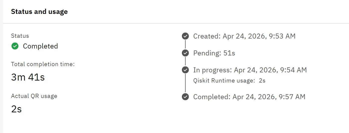
QAMOO job submitted to ibm_fez, April 24, 2026. Total completion time 3m 41s. Actual Qiskit Runtime usage 2s. The delta is queue wait and backend provisioning overhead. The benchmark's wall-clock solve times include this infrastructure cost.

Quantum Circuit Diagram

The QAMO circuit submitted to ibm_fez, April 23, 2026. Each horizontal line is a qubit. Each column of gate operations is one unit of depth. This circuit has a depth of 1,158. See Appendix A: Circuit Depth for context on why depth is the binding constraint on current NISQ hardware.